Use Python and Google Trends to Forecast Your Top GSC Keywords

Google Search Console already gives SEO’s amazing historical data for how the queries you rank for are performing. Google Trends also is a useful platform that can give insights into a query’s relative popularity within Google’s system (by Geo) historically and a little forecasting for the future. What if we could begin to marry these two systems to find the overall search trend for your top ranking queries to understand what the near-term potential could be.

In this Python SEO tutorial, I’ll show you step by step how to create the framework for determining if your top queries are trending up, down, are flat, or don’t have enough data. This could help forecast query performance (by Geo) in the near term and help you find queries to create more content if trending up!

Note, the results vary heavily depending on your settings and how you calculate the trend. Be sure you understand these things before taking any action or having confidence in them. Also, be sure you understand how Google Trends works and what their metrics mean.

Not interested in the tutorial? Head straight for the app here!

Requirements and Assumptions

• Python 3 is installed locally or Google Colab, and basic Python syntax is understood.
• Google Search Console performance data “Queries.csv” export file.
• Understanding how Google Trends works and what the data means.

Import and Install Modules

• pytrends: module that connects to the Google Trends API
• JSON: handles the request from the Google Trends API which comes in JSON format
• time: for pausing the script to prevent blocking
• pandas: for storing the information in a table form

First, let’s install the pytrends module which you won’t like have already.  If you are using Google Colab put an exclamation mark at the beginning.

pip install pytrends

First, we very simply import the 4 modules listed above that the script requires.

import pandas as pd
import json
import time
from pytrends.request import TrendReq

Settings and GSC Dataframe Setup

Next, we declare some variables we’re going to be using. Please fill these in with a value.

• get_gsc_file: the GSC Queries.csv file name and location
• sortby: How you want the top n queries to be selected. Choices are “Clicks”, “Impressions”, “CTR”, or “Position”
• cutoff: How many top n queries you want to process. Keep to a reasonable amount, perhaps under 200 or Google may ban you. Feel free to test.
• pause: How many seconds between Google Trends calls. This helps with not being banned. 1 second should be min.
• timeframe = What span of data do you want Google Trends to return. Choices are “Today 1-m”, “Today 3-m”, or “Today 12-m”.
• geo: Two-letter code for which country you want to segment. Leave as empty quotes for World.

get_gsc_file = ""
sortby = ""
cutoff = ""
pause = ""
timeframe = ""
geo = ""

Now we import the Queries.csv file into a pandas dataframe, sort descending by whatever dimension you chose above, and select the top n with n being whatever cutoff value you chose above.

df = pd.read_csv(get_gsc_file, encoding='utf-8')
df.sort_values(by=[sortby], ascending=False, inplace=True)
df = df[:cutoff]

Now we create an empty dataframe (sortby will import GSC data from whatever metric you’re sorting by) that will hold our trending information along with a couple of lists and counters for stats.

d = {'Keyword': [], sortby:[], 'Trend': []}
df3 = pd.DataFrame(data=d)
keywords = []
trends = []
metric = df[sortby].tolist()
up = 0
down = 0
flat = 0
na = 0

Process the GSC queries

Next, we iterate through the dataframe storing our GSC Queries data. Each row is a different query. We then initialize the TrendReq() function from pytrends and feed the keyword into the build_payload() function using some of the options we valued earlier. Lastly, we store the trend results given by the function interest_over_time() into a new dataframe named df2, and append that keyword to the keywords list.

for index, row in df.iterrows():
  keyword = row['Top queries']
  pytrends = TrendReq(hl='en-US', tz=360)
  kw_list = [keyword]
  pytrends.build_payload(kw_list, cat=0, timeframe=timeframe, geo=geo, gprop='')
  df2 = pytrends.interest_over_time()
  keywords.append(keyword)

Continuing inside the current loop using the trend data for the current keyword stored in df2, it’s now time to determine whether the trend is going up, going down, is flat or sometimes there is not enough data. There are many ways to determine this, so feel free to experiment. I chose to determine the trend of the last 5 weeks of data by averaging each week in sets of 3.

Once we have the 3 averaged trend points for the past 5 weeks, we can compare them against themselves in succession. Again, plenty of ways to modify this logic. Once we evaluate the trend, we can add the label to our trends list and increase the respective counter. Lastly, we need to pause the script for n seconds to not make Google Trends API mad.

try:
  trend1 = int((df2[keyword][-5] + df2[keyword][-4] + df2[keyword][-3])/3)
  trend2 = int((df2[keyword][-4] + df2[keyword][-3] + df2[keyword][-2])/3)
  trend3 = int((df2[keyword][-3] + df2[keyword][-2] + df2[keyword][-1])/3)

  if trend3 > trend2 and trend2 > trend1:
    trends.append('UP')
    up+=1
  elif trend3 < trend2 and trend2 < trend1:
    trends.append('DOWN')
    down+=1
  else:
    trends.append('FLAT')
    flat+=1
except:
  trends.append('N/A')
  na+=1
time.sleep(pause)

Build final dataframe and stats

When all the queries in the dataframe have been evaluated it’s time to dump them, the respective trends, and the GSC metric data you sorted by, into the empty dataframe df3 that we created earlier.

df3['Keyword'] = keywords
df3['Trend'] = trends
df3[sortby] = metric

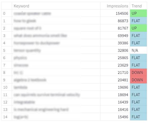
All the heavy lifting is now done and this next part is a bit optional. For fun, I decided to color-code the trends for easier dataframe scanning. This function applies a color based on the keyword trend value. Feel free to change colors and even style beyond this.

def colortable(val):
    if val == 'DOWN':
        color="lightcoral"
    elif val == 'UP':
        color = "lightgreen"
    elif val == 'FLAT':
        color = "lightblue"
    else:
        color = 'white'
    return 'background-color: %s' % color

 df3 = df3.style.applymap(colortable)

Next, I decided a few global stats are in order. Admittedly this is sloppy and it’s best itself in a dataframe. But if you want to output this in a quick and dirty matter. Here ya go! It’s just simple percentage formulas, with some rounding, string concatenation, and typing. Finally, we output the dataframe containing our keywords and color-coded trends.

total = len(trends)
print("Up: " + str(up) + " | " + str(round((up/total)*100,0)) + "%")
print("Down: " + str(down) + " | " + str(round((down/total)*100,0)) + "%")
print("Flat: " + str(flat) + " | " + str(round((flat/total)*100,0)) + "%")
print("N/A: " + str(na) + " | " + str(round((na/total)*100,0)) + "%")

df3

Sample Output

Conclusion

Now you have the framework to begin marrying GSC and Google Trend data together to inform on trends with keywords you’re ranking well for. Lots more potential on this one!

Don’t forget to try the streamlit app here!

Now get out there and try it out! Follow me on Twitter and let me know your Python SEO applications and ideas!

SEO Trend Forecasting FAQ