Classify Anchor Text N-Grams for Interlinking Insights with Python

In this Python SEO tutorial, I’ll show you a programmatic method to start analyzing your internal anchor text for topical relevance. Internal anchor text remains one of the most powerful topical endorsements you can provide. Anchor texts are explicit contextual signals Google can use to help understand and calculate the linked page’s topical authority. Let’s find out just how topically dense the signals in your anchor text are.

Like most of my SEO tutorials, I will give you a framework and starting point. There are countless approaches, extensions, and further drill-downs for complete analysis. The steps will be as follows:

1. Export an ahrefs internal links report (you could also modify using another platform export like DeepCrawl or even ScreamingFrog)
2. Clean the data
3. N-gram the anchor texts
4. Sort by n-gram frequency
5. Use Huggingface machine learning to classify
6. Graph the results

Requirements and Assumptions

• Python 3 is installed and basic Python syntax understood
• Access to a Linux installation (I recommend Ubuntu) or Google Colab.
• Very Basic NLP understanding

Import and Install Python Modules

• nltk: NLP module handles the n-graming and word type tagging
  • nltk.download(‘punkt’): functions for n-grams
  • nltk.download(‘stopwords’): contains a list of common stop words
• pandas: for storing and displaying the results
• string: for filtering out punctuation from the anchor text
• collections: for counting n-gram frequency
• transformers: machine learning algorithm for anchor text classification

Let’s first install the Huggingface transformers module we’ll use for the classification step. If you’re using Google Colab remember to put an exclamation point at the beginning.

pip3 install transformers

Now we’ll import all the modules I listed above.

import pandas as pd
import nltk
nltk.download('punkt')
from nltk.util import ngrams
from nltk.corpus import stopwords
nltk.download('stopwords')
import string
from collections import Counter
from transformers import pipeline

Next, we need to import the ahrefs internal link report CSV into a dataframe. The CSV in Sheets should look like this format. We will only be using the “outbound-anchor” column.

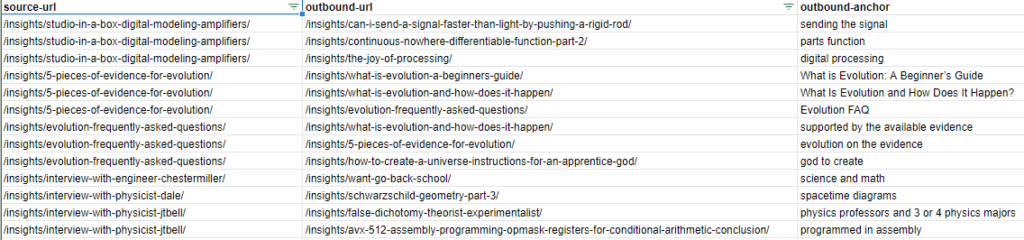
df = pd.read_csv("ngrams.csv")
df

Create N-gram Functions

This next snippet of code is the function to n-gram the anchor text. We take in all the anchors as a string, provide the number of grams we want (1 or 2 is best) and then send them to the NLTK module for processing and what is returned is the list of n-grams.

def extract_ngrams(data, num):
  n_grams = ngrams(nltk.word_tokenize(data), num)
  gram_list = [ ' '.join(grams) for grams in n_grams]
  return gram_list

Below we take all the anchors texts in the dataframe, put them into a list, and convert them all to string so we don’t mix data types when we n-gram. Then we join all the anchor texts into one large string and send it to the function we created above to be n-gramed. After the result is returned we do a little data clean-up. We lowercase all the n-grams and filter out punctuation and stop words.

anchors = [str(x) for x in df['outbound-anchor'].tolist()]
data = ''
data = ' '.join(anchors)
keywords = extract_ngrams(data, 2)
keywords = [x.lower() for x in keywords if x not in string.punctuation]
keywords = [x for x in keywords if ":" not in x]
stop_words = set(stopwords.words('english'))
keywords = [x for x in keywords if not x in stop_words]

Once we have our cleaned n-gram list we can easily calculate the frequency using the Counter() function in the Collections module. The number in the function can be used to limit how many are calculated. Then we create a dataframe containing those keywords and counts. It should look similar to the dataframe below (but much longer). It’s important to remember that these aren’t always full anchor texts. They are slices intended to classify to determine how topically dense they are, which we are doing next.

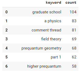
Sort N-gram frequency

keywords = list(Counter(keywords).most_common(100))

df2 = pd.DataFrame(keywords,columns=["keyword","count"])
df2

Now that we have our bi-gram’d anchor texts we can attempt to classify via a curated topics list that you can create yourself. My site is physics-based so I decided on 6 categories. In order to catch poor anchor text signals, I also include one called “random” which the model often uses when something doesn’t at all fit other categories. The model we’re using is distilbart-mnli-12-9 and is from Huggingface. It’s a zero-shot-classification model meaning that the dataset the model was trained on won’t be specific to our data. I have a full tutorial on the distilbart model here.

Categorize N-gram with machine learning

topics =['education','physics','astronomy','math','engineering','random']
classifier = pipeline("zero-shot-classification",
                      model="valhalla/distilbart-mnli-12-9")

Once we have our categories set and the model loaded (often over 1gig) we can create the empty lists that will hold the results of each anchor text n-gram processed by the classification model. The loop iterates through the anchor text column, sending the anchor and topic categories to the model. The results are in JSON form so we can easily parse to find the top-scored topic since it evaluates each. Then we simply add the top score and topic to the empty lists we created earlier, rinse and repeat.

topic_list = []
topic_list_score = []

### iterate through crawl dataframe
for index, row in df2.iterrows():

  #### parent topic generation
  sequence_to_classify = row[0].lower()
  result = classifier(sequence_to_classify, topics)

  ### parse results, select top scoring result
  topic = result["labels"][0]
  topic_score = str(round(result["scores"][0],3))

  ### add result to topic list
  topic_list.append(topic)
  topic_list_score.append(topic_score)

Now we simply add the new topics per anchor text n-gram to the dataframe.

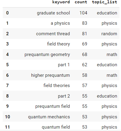
df2["topic_list"] = topic_list
df2

Graph categories

If you have a small number of anchor texts you may just be able to browse through the rows and get a feel for what is optimal and what isn’t. In the case where you have a large site and could use a visual, we’ll take this extra step and graph our categorical buckets.

We first need to make sure the data is typeset correctly before graphing, then we sum the counts of each topic group in the dataframe and send the data to the bar() plot function.

df2["count"] = df2["count"].astype(float)
df2["topic_list"] = df2["topic_list"].astype(str)

df2 = df2.groupby(['topic_list'])['count'].sum().to_frame().sort_values('count', ascending=False).reset_index()
df2.plot.bar(x='topic_list', y='count',figsize=(15,5), title="Anchor Categories", xlabel="Category", ylabel="Count", rot=20)

Output and Conclusion

It doesn’t take a data scientist to see that I’ve got a problem with my anchor text topical relevance. There are a lot of n-grams that are classified under the random category. The next step would be to examine this bucket further and see where I can improve where these n-grams are actually in anchor text. Anchor text should not be taken for granted and be a strong player in your SEO strategy. Every anchor text should be carefully created with maximum topical relevance signals in mind.

Now you have the start of a framework to begin understanding what topical signals and the strength of those signals are within your anchor text. Remember to try and make my code even more efficient and extend it in ways I never thought of!  Now get out there and try it out! Follow me on Twitter and let me know your applications and ideas!

N-Gram Interlinking FAQ

How can Python be utilized to classify anchor text N-grams for gaining insights into interlinking strategies?

Python scripts can be developed to analyze anchor text N-grams, providing insights into the patterns and strategies employed for interlinking within a website.

Which Python libraries are commonly used for classifying anchor text N-grams?

Commonly used Python libraries for this task include nltk for natural language processing, pandas for data manipulation, and machine learning libraries like scikit-learn for classification.

What specific steps are involved in using Python to classify anchor text N-grams for interlinking insights?

The process includes fetching anchor text data, preprocessing the text, extracting N-grams, classifying the N-grams based on predefined criteria, and using Python functions for analysis.

Are there any considerations or limitations when using Python for this classification?

Consider the diversity of anchor text, potential biases in the training data, and the need for a clear understanding of the goals and criteria for classification. Regular updates to the classification model may be necessary.

Where can I find examples and documentation for classifying anchor text N-grams with Python?

Explore online tutorials, documentation for relevant Python libraries, and resources specific to natural language processing and machine learning for practical examples and detailed guides on classifying anchor text N-grams using Python.