Find Search Volume Ceiling for Keyword Categories Using Python

In this tutorial I’ll show how to use Python to generate broad keyword categories from current ranking keyword data and automatically label keywords with those categories. This helps you get an overview of the topics you rank for and the potential search-volume ceilings for each category. The largest opportunities often appear in categories with the highest total volume ceilings. These potential search volumes estimate an upper bound — what you could expect if you ranked #1 for every keyword and every user clicked your link. While not realistic, this upper-bound data is a useful reference.

Requirements and Assumptions

• Python 3 is installed and you understand basic Python syntax
• Access to a Linux installation (Ubuntu recommended) or Google Colab.
• Keyword data with search volume (e.g., Semrush organic research export)

Import Modules and Data Table Extension

Let’s start by importing pandas and the Google Colab data table extension (for easier DataFrame viewing).

import pandas as pd
%load_ext google.colab.data_table

Now load the CSV keyword data into two different DataFrames. Although it’s possible to do everything we need using a single DataFrame, using two was simplest for me. The first DataFrame only needs the Keyword column to generate the word counts we’ll use to auto-label keywords into categories.

df = pd.read_csv("rckey.csv")['Keyword']
df2 = pd.read_csv("rckey.csv")

With the keyword data loaded in both DataFrames, we’ll start with the first to generate the keyword categories. The Keyword column contains phrases, so we split() each phrase on whitespace to create lists, use explode() to turn those words into rows, count the unique words in that column, and reset the DataFrame index.

df = df.str.split().explode().value_counts().reset_index()

This column likely contains many stop words; filter those out and add words to the list as needed.

stop = ['1','2','3','4','5','6','7','8','9','get','ourselves', 'hers','us','there','you','for','that','as','between', 'yourself', 'but', 'again', 'there', 'about', 'once', 'during', 'out', 'very', 'having', 'with', 'they', 'own', 'an', 'be', 'some', 'for', 'do', 'its', 'yours', 'such', 'into', 'of', 'most', 'itself', 'other', 'off', 'is', 's', 'am', 'or', 'who', 'as', 'from', 'him', 'each', 'the', 'themselves', 'until', 'below', 'are', 'we', 'these', 'your', 'his', 'through', 'don', 'nor', 'me', 'were', 'her', 'more', 'himself', 'this', 'down', 'should', 'our', 'their', 'while', 'above', 'both', 'up', 'to', 'ours', 'had', 'she', 'all', 'no', 'when', 'at', 'any', 'before', 'them', 'same', 'and', 'been', 'have', 'in', 'will', 'on', 'does', 'yourselves', 'then', 'that', 'because', 'what', 'over', 'why', 'so', 'can', 'did', 'not', 'now', 'under', 'he', 'you', 'herself', 'has', 'just', 'where', 'too', 'only', 'myself', 'which', 'those', 'i', 'after', 'few', 'whom', 't', 'being', 'if', 'theirs', 'my', 'against', 'a', 'by', 'doing', 'it', 'how', 'further', 'was', 'here', 'than']

df = df[~df['index'].isin(stop)].reset_index()

Next, take the top 20 keyword categories and put them in a list. You can change this number or omit it if you’re saving to a spreadsheet, but 20 works well for charting.

topkeywords = df['index'][:20].to_list()
print(topkeywords)

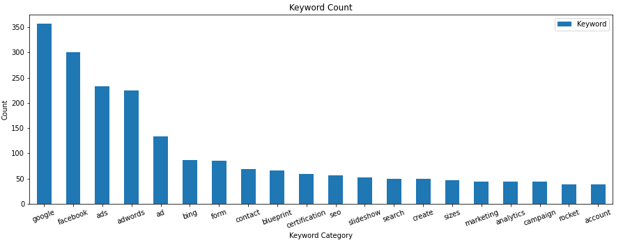
Let’s make a quick chart of the counts for each keyword category.

df[:20].plot.bar(y='Keyword', x='index', figsize=(15,5), title="Volume", rot=20)

Next we’ll label keywords with the categories so we can sum their search volumes, using the second DataFrame. The extract() function searches the Keyword column with a regex and, on a match, places the result in a new Marked column. We build the regex from the categories generated earlier; the variable regex will look like “word1|word2|word3|…” when using join(). Rows without matches are dropped with dropna().

regex = '(' + ('|'.join(topkeywords)) + ')'
df2['Marked'] = df2.Keyword.str.extract(regex)
df2 = df2.dropna()

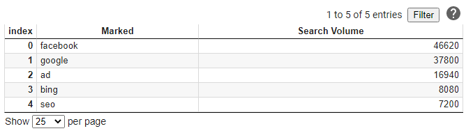
Now group identical keyword categories, sum their Search Volume, and sort by Search Volume descending.

df2 = df2.groupby(['Marked'])['Search Volume'].sum().to_frame().sort_values('Search Volume', ascending=False).reset_index()
df2.head()

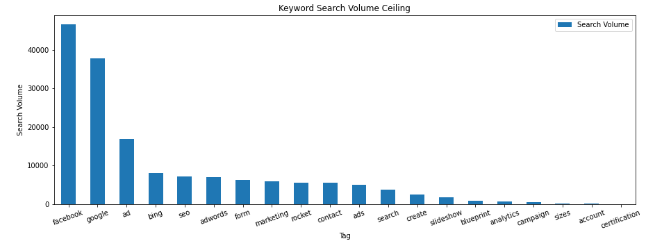
Finally, plot these columns to visualize the potential volumes for the keywords you rank for.

df2.plot.bar(y='Search Volume', x='Marked', figsize=(15,5), title="Keyword Search Volume Ceiling", xlabel="Tag", ylabel="Search Volume", rot=20)

Conclusion

With this framework, you can generate keyword categories and summed search volumes for any website to identify opportunities. In the next tutorial I’ll show how to apply this to landing page data and sessions. Try it out, and follow me on Twitter to share your applications and ideas!